This is your first blog of the ohsome series? Before you might be confronted with any potential spoilers, you should better check out the first and the second part of this blog series (or the intro to the idea and general architecture) to be on the safe side and up to date with the current content.
So here we are again, back with a new blog of the how to become ohsome series. As promised last time, we will take a look at different mapping/tagging schemes. Therefore, we will query OpenStreetMap (OSM) history data from two different cities and compare the usage of the building tag. The chosen cities are both of similar size (roughly 150k inhabitants), but situated in two different European countries: Salzburg in Austria and Oxford in Great Britain. We will use the elements/count/groupBy/tag resource of the ohsome API to get our results grouped on different tags. Speaking of tags, we use the four most frequent building tags from taginfo: yes, house, residential and garage. The requests are built with the following parameters:
bpolys=[respective GeoJSON FeatureCollection]
time=2010-01-01/2018-07-01/P6M
format=csv
types=way
keys=building
groupByKey=building
groupByValues=yes,residential,house,garage
Our two requests contain the spatial component bpolys, having the two GeoJSON boundaries from our two regions, one for each request. You can derive these boundaries, or any other boundary from this website.
The temporal parameter time describes a time frame from 2010-01-01 to 2018-07-01 in a half-year interval (P6M stands for 6 months). This means we will get 18 results, two for every year at the first of January and the first of July respectively.
The format=csv parameter tells the API that we are interested in getting a csv file as a response, which we want to load directly into a spreadsheet program, e.g. Excel.
The types and keys parameters are our first two attributive filters, explaining that we want to query OSM way features that have any building tag assigned to them. Via the last two attributive parameters groupByKey and groupByValues, we define on which tags the grouping should be based.
Please also notice the naming of the parameters in respect to singular vs. plural: Parameters like format, or groupByKey can only contain zero or one value, whereas others like keys, or groupByValues can contain zero or more.
To make your life tweaking the API easier, we’ve created another snippet that includes the cURL requests, the parameters, as just described, as well as a view on one of the returned responses.
After the responses are returned, we can load the content into our spreadsheet program and create the following two diagrams:
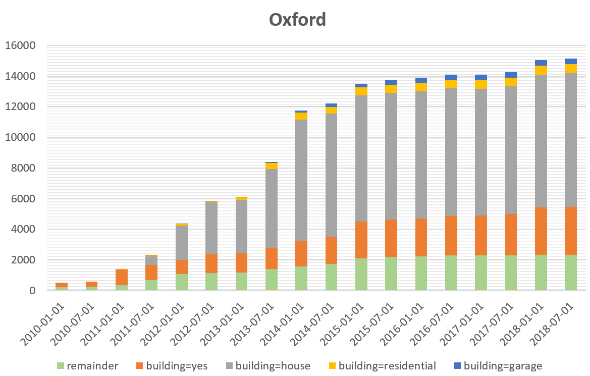
The first one shows the number of buildings having the requested tags for Oxford. Additionally to the 4 tags, we see a category called remainder, which represents the number for all other building tags. Looking at the results, the most used building tag since 2012 is building=house, where it surpassed the second most frequent building=yes tag.
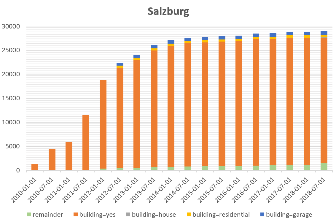
The second diagram gives us the numbers for Salzburg. What probably jumps into one’s eyes at first sight are the long orange bars referring to the tag building=yes. This generic tag takes by far the biggest margin of the visualized tag distribution, having between 1300 and 26000 occurrences at the requested timestamps. In comparison to that, building=house only has between 0 and 132 occurrences.
In this 3rd part of how to become ohsome, we’ve demonstrated how you can take a look at different tagging schemes through using the ohsome API to query OSM’s history. You want to learn more about how to use our ohsome framework? Take a look at other blog posts (1, 2, 3, 4, 5).
You want to give us feedback? Just write an email to info@heigit.org. You want to know something about the next blog post? Subscribe to our ohsome blog posts using this link to the rss feed. The next episode might tell you how to analyze historical OSM data on a global scale. So stay tuned 😉