This blog post introduces a step-by-step tutorial for working with a global road surface dataset. Using open-source tools, the tutorial demonstrates how to identify infrastructure gaps by combining road surface data with population information.
How much time does a humanitarian mission need to reach a remote village after a cyclone hits rural Madagascar? How fast can a woman in labor reach the nearest hospital during monsoon flooding in southern Pakistan? What is the logistical cost of transporting agricultural goods from unpaved rural roads in Zambia to the nearest trade hub? How vulnerable are supply chains in Southeast Asia to climate-related disruptions on poor-quality road networks? And the list goes on.
These questions are at the heart of planning and decision-making in disaster response, transportation logistics, and sustainable development. To answer them, you need more than just a map. You need to understand the actual condition of the roads. That’s where road surface data comes in. Combined with tools for spatial analysis and other open-source datasets, it offers more targeted, and evidence-based insights.
Road surface dataset
The road surface dataset provides information on road conditions worldwide, distinguishing between paved and unpaved surfaces. It is built upon OpenStreetMap (OSM) road geometries and enhances them using a GeoAI pipeline that draws from over 105 million crowdsourced images contributed via Mapillary. The processing approach combines SWIN-Transformer-based surface classification with CLIP-assisted filtering to exclude poor-quality imagery, ensuring high reliability of predictions.
Currently, only about 33% of roads in OSM include any surface type information with data gaps being especially pronounced in developing regions. To help address this, HeiGIT has released a global dataset covering approximately 36.7 million kilometers of roads, expanding the availability of surface type data to around 36% of the global road network. This represents a substantial improvement in coverage, with further enrichment planned through the integration of satellite imagery to close remaining data gaps.
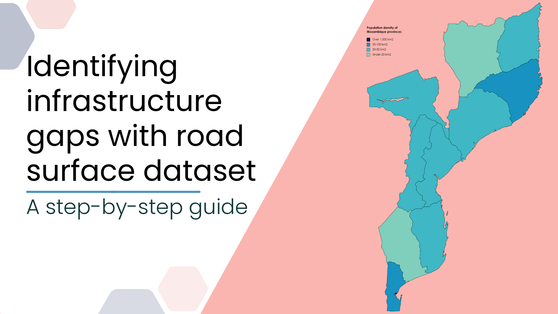
Tutorial: a case study in Mozambique
This tutorial demonstrates how to use the road surface dataset in a real-world scenario, focusing on a case study in Mozambique. We show how to integrate the road surface data with global population data using geospatial tools such as DuckDB, Mercantile, and Shapely. The case study highlights areas with incomplete or missing surface information, particularly in rural regions, and demonstrates how such insights can support applications in accessibility analysis, infrastructure planning, and emergency logistics.
We have divided the tutorial into two parts:
In Part I, we demonstrate how to perform efficient spatial joins in DuckDB by simulating a spatial index with tile-based filtering, enabling faster matching of road features to geographic regions.
In Part II, we show how to aggregate road surface prediction results by tile, computing total lengths, coverage ratios, and counts of predicted vs. OSM road segments, and exports the statistics as a Parquet file.
Part I
For this we will show how to:
- Generate vector tiles from polygons using Mercantile,
- Register custom Python functions inside DuckDB, and
- Set up a geospatial processing workflow that’s fast, flexible, and reproducible.
Getting started: imports
If you’re running this locally, make sure the required packages are installed. You can uncomment the lines below to install them:
#!pip install duckdb
#!pip install mercantile
#!pip install shapely

import os
import mercantile
import duckdb
from shapely import from_wkt, to_wkt, box
To analyze spatial data tile-by-tile, we first need to convert tile coordinates (z, x, y) into geometries. Mercantile allows us to compute the bounding box of a tile, and Shapely can then turn that box into a polygon.
def create_tile(tile_wkt):
    numbers = [int(x) for x in tile_wkt[1:-1].split(',')]
    bbox = mercantile.bounds(*numbers)
    return to_wkt(box(*bbox))
Generating tile lists from polygons
Working with global datasets like road networks and population layers poses a major challenge: they are too large to handle in a single query or to load fully into memory. To address this, we split the problem into smaller, spatially bounded chunks.
Given a geographic polygon (like a country border or region of interest), we often want to find all the map tiles that intersect it at a given zoom level. This step links spatial data to specific geographic areas. The function used here returns a list of tile coordinates that cover the bounding box of any given polygon.
def finding_tiles_list_for_areas(polygon_str, zoom_level):
    bbox = from_wkt(polygon_str).bounds
    return ['[' + ','.join([str(int(tl.x)), str(int(tl.y)), str(int(tl.z))]) + ']'
            for tl in list(mercantile.tiles(*bbox, zoom_level))]
Setting up your working directory and parameters
Before running the analysis, change to the working directory and define key input & output files and zoom level. You can adjust these parameters to match your local environment and data sources. Change ‘main_dir’ to your working directory where the input files (‘filename’, ‘polygons_filename’) are located and modify the names of these filenames below to your own files.
main_dir = 'D:/work-heigit/mapillary_data_extraction/tutorial'
os.chdir(main_dir)

zoom_level = 14
filename = 'heigit_moz_roadsurface_lines.gpkg'
polygons_filename = 'EMSR495_AOI01_DEL_MONIT03_observedEventA_r1_v1.shp'
output_filename = 'intersected_file.parquet'
stats_output_filename = 'final_stats.parquet'
Enabling spatial functions in DuckDB
Install and load the spatial extension in DuckDB to enable GIS operations. DuckDB is a light SQL programming environment, known for its versatility, ease of use and speed.
duckdb.sql("INSTALL spatial; LOAD spatial;")Registering Python functions in DuckDB
Use duckdb.create_function() to make the two custom Python functions available in SQL queries. Beside the default functions and as well as those that are available in different packages, DuckDB also allows the definition of custom Python functions to be used in queries. To do this
We first provide a name for these functions, followed by the Python function itself. The list [‘varchar’, ‘double’] specify the datatypes of the inputs. The second string following this specifies the format of the output. ‘varchar’ stands for string, whereas ‘double’ for numerical values. ‘varchar[]’ means that the output is a list of strings.
duckdb.create_function("finding_tiles_list_for_areas", finding_tiles_list_for_areas, ['varchar','double'], 'varchar[]')C:\Users\admin\AppData\Local\Temp\ipykernel_2228\1876444308.py:1: DeprecationWarning: numpy.core is deprecated and has been renamed to numpy._core. The numpy._core namespace contains private NumPy internals and its use is discouraged, as NumPy internals can change without warning in any release. In practice, most real-world usage of numpy.core is to access functionality in the public NumPy API. If that is the case, use the public NumPy API. If not, you are using NumPy internals. If you would still like to access an internal attribute, use numpy._core.multiarray.
duckdb.create_function("finding_tiles_list_for_areas", finding_tiles_list_for_areas, ['varchar','double'], 'varchar[]')
<duckdb.duckdb.DuckDBPyConnection at 0x1727e69a9f0>Performing spatial joins with DuckDB
This section walks through a multi-step SQL query that matches road features to geographic regions using tile-based filtering. Since DuckDB does not currently support spatial indexes, we simulate one using tile intersections to reduce computational overhead.
The logic unfolds in several steps:
- We only retrieve the IDs and geometries from our file in case the file is big so that we do not have any memory issues. This is the table ‘data’. We also use our custom function ‘finding_tiles_list_for_areas’ to assign the corresponding tiles on zoom level ‘z’ to use them later to find intersections. This will kind of function as a spatial index as duckDB does not support spatial indexing as of yet.
- We open our ‘polygons_filename’, assign their row number as their ID and do the same tiles finding operation on our polygons as well.
- DuckDB will conceptually start with all possible
datarows (a) andpolygonsrows (b) when evaluating theLEFT JOIN. However, instead of directly checkingST_Intersectson every pair (which would be expensive), theONclause ensures that two conditions must be true for a match: 1) Tile overlap check —list_has_any(...)— this quickly determines whether the tile index lists foraandbshare at least one common tile. 2) Geometry intersection check —ST_Intersects(...)– Only if the tile overlap isTRUEdoes DuckDB then check actual polygon vs. geometry intersection. - We check whether the elements of
dataandpolygonshave any intersections via the default duckdBlist_has_any()function and only in the affirmative case, we intersect the corresponding geometries with one another viaST_Intersects()function. By doing this, we reduce the amount of spatial intersections we have to carry out. Thereafter, we save the relevant columns from both tables via aLEFT JOIN. This is theintersectiontable.
- Having carried out the intersections, we can now go back to our file and retrieve the whole data from ‘filename’ of only those rows that were located in the provided ‘polygons_filename’ file. This is done in table ‘all_cols_data’
- Having retrieved whole data, we only have to carry out a second join to add the information coming from the polygons to the data. This is done in the last ‘SELECT’ clause.
query = f"""
COPY(
    WITH
    -- we select only the ID and Geometry column from the country file in case it is too big to store in the memory
    -- we'll apply our intersection logic only on these columns. We'll use IDs, later on, to read the qualifying data from the main
    -- country file

    --here, we create grids on some zoom level for the main data, so that we can compare the tiles the main data intersects with those from the polygons, i.e. spatial indexing
    --because, Duckdb does not offer any spatial indexing
    data AS(
        SELECT osm_id, geom,
            finding_tiles_list_for_areas(ST_AsText(geom), {zoom_level}) as z_lvl_{int(zoom_level)}_tiles
        FROM '{filename}'
    ),

    --we add the row number as an ID column for the polygons and we do the same 'spatial indexing' for the polygons
    polygons AS(
        SELECT *,
            ROW_NUMBER() OVER () as polygon_id,
            finding_tiles_list_for_areas(ST_AsText(geom), {zoom_level}) as z_lvl_{int(zoom_level)}_tiles
        FROM '{polygons_filename}'
    ),

    --here, we carry out a 'join' operation between the main data and the polygons. First, we compare, whether the tiles list of a main data row has any tiles in common with any polgon ('list_has_any()' function)
    --only in the case that there is at least one tile, we intersect the data geometry with that of the corresponding polygon. This reduces the geometric operations substantially
    --we also save the ID columns as well as polygon geometries so that we can use them in the next step.
    intersection AS(
        SELECT
            a.osm_id,
            b.polygon_id,
            b.geom as polygon_geom,
            list_intersect(a.z_lvl_{int(zoom_level)}_tiles, b.z_lvl_{int(zoom_level)}_tiles) as intersected_tiles
        FROM data a
        LEFT JOIN polygons b
            ON list_has_any(a.z_lvl_{int(zoom_level)}_tiles, b.z_lvl_{int(zoom_level)}_tiles)
            AND ST_Intersects(a.geom, b.geom)
    ),

    --here, we select all columns from the data file for those rows only that intersect some polygons
    all_cols_data AS(
        SELECT *
        FROM '{filename}'
        WHERE osm_id IN (SELECT osm_id
                     FROM intersection
                     WHERE polygon_id IS NOT NULL
                     )
    )

    -- we carry out a second 'join' operation to merge the all column data with intersections
    SELECT
        a.* REPLACE(ST_Intersection(a.geom, b.polygon_geom)) as geom,
        b.polygon_id,
        ST_AsText(b.polygon_geom) as polygon_geom,
        UNNEST(b.intersected_tiles) as z_lvl_{int(zoom_level)}_tile
        FROM all_cols_data a
        LEFT JOIN intersection b
            ON a.osm_id = b.osm_id
)
TO '{output_filename}'
(FORMAT 'parquet', COMPRESSION 'zstd');
"""
duckdb.sql(query)
Given your query, the result will have:
| Column name | Source table | Description |
|---|---|---|
| osm_id | a (data) | The OSM ID of the feature from the main dataset. |
| polygon_id | b (polygons) | The unique ID of the polygon that matched via tile + geometry intersection. Will be NULL if no polygon matched. |
| polygon_geom | b (polygons) | The geometry of the matching polygon. Will be NULL if no polygon matched. |
| intersected_tiles | computed | A list containing only the tile IDs that are present in both a.z_lvl_{zoom_level}_tiles and b.z_lvl_{zoom_level}_tiles. Will be NULL if no match. |
| osm_id | polygon_id | polygon_geom | intersected_tiles |
|---|---|---|---|
| 12345 | P001 | POLYGON(…) | [T1234, T5678] |
| 12346 | NULL | NULL | NULL |
| 12347 | P002 | POLYGON(…) | [T3456] |
PART II
Aggregating road surface prediction statistics
Once the spatial join is complete, we can begin analyzing coverage and quality of the road surface predictions. This query summarizes the dataset by calculating:
- The percentage of road segments with surface predictions
- (variable:
predicted_pct)
- (variable:
- Their total length
- (variables:
total_predicted_length,total_predicted_paved_length,total_predicted_unpaved_length,total_osm_length)
- (variables:
- Optionally, breakdowns by polygon (e.g., districts) or highway type (primary, residential, etc.)
- (variables:
grouped_by_polygon,grouped_by_highway_type)
- (variables:
By commenting (adding — at the start of a line) uncommenting (deleting — at the start) the relevant parts at the start and end of the query, the stats can also be constructed on the polygon level given by ‘polygon_id’. For both aggregation levels, the stats can also be created for each OSM highway type individually if wished so.
stats_query = f"""
COPY(
    SELECT
        z_lvl_{int(zoom_level)}_tile,
        --z_lvl_{int(zoom_level)}_tile, highway,
        --polygon_id,
        --polygon_id, highway,
        -----------------------------calculation of lengths--------------------------------------
        SUM(CASE WHEN predicted_length IS NOT NULL THEN predicted_length ELSE 0 END) as total_predicted_length,

        SUM(CASE WHEN pred_label = 0 THEN predicted_length ELSE 0 END) as total_predicted_paved_length,

        SUM(CASE WHEN pred_label = 1 THEN predicted_length ELSE 0 END) as total_predicted_unpaved_length,

        SUM(CASE WHEN osm_length IS NOT NULL THEN osm_length ELSE 0 END) as total_osm_length,
        -----------------------------------------------------------------------------------------

        -------------------------------calculation of predicted length coverage -----------------
        SUM(CASE WHEN predicted_length IS NOT NULL THEN predicted_length ELSE 0 END) /
        SUM(CASE WHEN osm_length IS NOT NULL THEN osm_length ELSE 0 END) as predicted_length_ratio,

        SUM(CASE WHEN pred_label = 0 THEN predicted_length ELSE 0 END) /
        SUM(CASE WHEN osm_length IS NOT NULL THEN osm_length ELSE 0 END) as predicted_paved_length_ratio,

        SUM(CASE WHEN pred_label = 1 THEN predicted_length ELSE 0 END) /
        SUM(CASE WHEN osm_length IS NOT NULL THEN osm_length ELSE 0 END) as predicted_unpaved_length_ratio,
        -----------------------------------------------------------------------------------------

        ------------------------- calculation of predicted osm_ids ------------------------------
        COUNT(DISTINCT CASE WHEN pred_label IS NOT NULL THEN osm_id ELSE NULL END) as n_of_predicted_osm_ids,

        COUNT(DISTINCT CASE WHEN pred_label = 0 THEN osm_id ELSE NULL END) as n_of_predicted_paved_osm_ids,

        COUNT(DISTINCT CASE WHEN pred_label = 1 THEN osm_id ELSE NULL END) as n_of_predicted_unpaved_osm_ids,

        COUNT(DISTINCT osm_id) as n_of_osm_ids,

        -------------------------------calculation of predicted OSM ID coverage ------------------
        COUNT(DISTINCT CASE WHEN pred_label IS NOT NULL THEN osm_id ELSE NULL END) /
        COUNT(DISTINCT osm_id) as predicted_osm_id_ratio,

        COUNT(DISTINCT CASE WHEN pred_label = 0 THEN osm_id ELSE NULL END)/
        COUNT(DISTINCT osm_id) as predicted_paved_osm_id_ratio,

        COUNT(DISTINCT CASE WHEN pred_label = 1 THEN osm_id ELSE NULL END)/
        COUNT(DISTINCT osm_id) as predicted_unpaved_osm_id_ratio,

        ST_GeomFromText(create_tile(z_lvl_{int(zoom_level)}_tile)) as geom
        --ST_GeomFromText(ANY_VALUE(polygon_geom)) as geom
    FROM '{output_filename}'
    GROUP BY z_lvl_{int(zoom_level)}_tile
    --GROUP BY z_lvl_{int(zoom_level)}_tile, highway
    --GROUP BY polygon_id
    --GROUP BY polygon_id, highway
)
TO '{stats_output_filename}'
(FORMAT 'parquet', COMPRESSION 'zstd');
"""
df = duckdb.sql(stats_query)
The combination of these two datasets helps answer questions such as:
- Which districts in Mozambique have many people but poor road conditions?
- How much of the road infrastructure used by the population is actually documented in OSM?
- Where could additional surface data change the picture of accessibility?
This tutorial focused on identifying infrastructure gaps in Mozambique — just one of many potential applications of the road surface dataset. When combined with other open datasets, such as population grids, health facility locations, or climate vulnerability indices, it can help answer complex questions across sectors. From modeling rural accessibility and evaluating climate resilience, to optimizing logistics or guiding investment in road infrastructure, the dataset offers a flexible foundation for research, policy, and decision-making.
We encourage you explore new combinations of data, and share your findings. The more perspectives and use cases we gather, the better we can understand how to close the remaining gaps. If you want to share your use-case, reach out to: communications[at]heigit.org
Stay tuned for our upcoming paper and dataset on road surface classification from satellite imagery, where we provide global coverage of all critical roads with high accuracy!
Datasets: HeiGIT (Heidelberg Institute for Geoinformation Technology) Humanitarian Data | 231 Datasets | HDX
Research paper: Randhawa, S., Aygün, E., Randhawa, G., Herfort, B., Lautenbach, S., & Zipf, A. (2025). Paved or unpaved? A deep learning derived road surface global dataset from mapillary street-view imagery. ISPRS Journal of Photogrammetry and Remote Sensing, 223, 362–374. https://doi.org/10.1016/j.isprsjprs.2025.02.020
Image source: File:Population density of Mozambique provinces.png


