The Climate Action Navigator (CAN) is HeiGIT’s interactive dashboard offering high-resolution data and key climate indicators, ranging from the quality and availability of mobility infrastructure to CO2 emissions from heating of residential buildings.
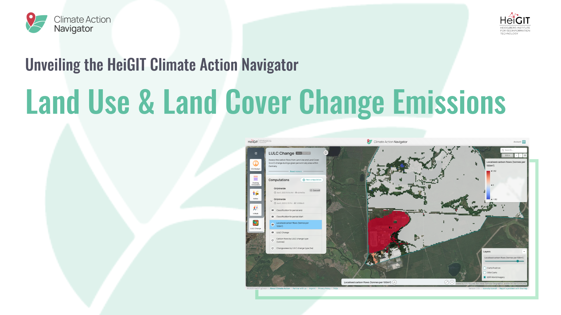
In this blog article, we will have a closer look at Land Use and Land Cover (LULC) Change Emissions. The LULC Change assessment tool provides high-resolution emission estimates for a custom time period at a spatial scale relevant to local climate-related policies and stakeholders.
Why information on LULC change emissions is crucial for climate mitigation
LULC change has been identified as a significant driver of CO2 emissions. Therefore, having detailed spatial information about these changes is crucial for identifying where the largest emissions occur. For example, when land is converted for agriculture, infrastructure, or urban development, it can lead to significant carbon releases. Efforts to reduce these emissions, such as promoting more sustainable land management practices, can sometimes create competing demands on land. However, with thoughtful planning, it is possible to implement solutions that balance environmental and socioeconomic needs. To explicitly plan such measures, high-resolution spatial information is required.
The LULC Change assessment tool: more than a LULC map
This LULC Change assessment tool is more than just a LULC change map. In addition to mapping land cover changes, it provides high-resolution estimates of the emissions caused by those changes, offering deeper insights into environmental impact. Furthermore, it is more practical than many existing LULC maps, due to its higher spatial and temporal resolution and its interactive design. Users can select specific timestamps and regions, enabling targeted, detailed analysis that supports more informed decision making.
Information on LULC change emissions from the dashboard can be used in several impactful ways. First, it allows users to identify key areas where LULC changes are resulting in significant emissions. This helps prioritize regions that may require closer monitoring or immediate intervention.
Second, the data can support local actors such as municipalities, environmental agencies, or land managers in quantifying their contributions to LULC-related emissions. This is essential for reporting, policy development, and tracking progress toward climate goals.
Finally, the tool can aid in planning effective emission mitigation measures. By understanding when and where emissions are occurring, stakeholders can design targeted strategies to reduce future impacts, improve land management practices, and support more sustainable development.
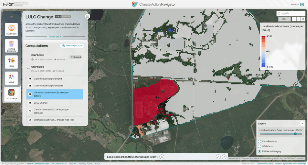
Screenshot of LULC Change Tool in CAN – This example shows Grünheide, Germany
How LULC Change works: methods and data
LULC Change Detection
To detect LULC changes, classifications from Sentinel 2 satellite images at the start and end of a selected period are compared. Computations are possible for time periods from 2017 onward. To obtain the LULC classifications, images from July of the respective year are used. For example, if the analysis period is 2017–2024, changes between July 2017 and July 2024 are assessed by identifying pixels that switch from one LULC class to another.
LULC classification from satellite imagery is subject to uncertainties, particularly due to cloud cover, atmospheric effects, and classification noise (e. g., salt-and-pepper artifacts or mixed pixels). To reduce the impact of such errors, only classifications with a model confidence of at least 75% are considered valid; those below this threshold are marked as “unknown”. The classification model is specifically trained for Germany, so the tool is currently restricted to use within this region. We plan to expand the tool to other regions in the future.
Carbon Flow Calculation
Carbon flows are estimated by comparing the carbon stocks associated with the initial and final LULC classes. These stocks account for both soil and vegetation carbon and represent average values per hectare. Different land types store different amounts of carbon: for instance, forests store more carbon than grasslands or urban areas. We use a specific carbon stock value for each land type to calculate the difference in carbon stocks between the start and end of the selected period. The result is an estimated carbon emission or sequestration value (measured in tonnes per hectare).
Users can choose from three data sources for carbon stock values:
- BLUE model (Hansis et al., 2015),
- Higher values from Hansis et al. (2015) based on Reick et al. (2010),
- CDIAC database (Houghton & Hackler, 2001).
These sources differ in assumptions, particularly regarding land use heterogeneity and the timing of carbon stock changes, leading to varying uncertainty levels in the results. For detailed assumptions and methods, please refer to the original publications.
From insight to action: the Climate Action Navigator
The Climate Action Navigator is more than just a dashboard to assess climate mitigation measures in cities worldwide. It aims to identify local strengths, highlight areas for improvement, and support the development of targeted solutions to make cities more livable, inclusive, and climate-resilient. Unlike traditional indices, the CAN assessment tools are co-created with urban planners, advocacy groups, and local stakeholders to ensure practical and actionable results.
More information on the Climate Action Navigator and its assessment tools can be found on the project webpage.
References
- Hansis, E., Davis, S. J., & Pongratz, J. (2015). Relevance of methodological choices for accounting of land use change carbon fluxes. Global Biogeochemical Cycles, 29(9), 1230–1246. https://doi.org/10.1002/2014GB004997
- Houghton, R. A., & Hackler, J. L. (2001). Carbon flux to the atmosphere from land-use changes: 1850 to 1990 (NDP-050/R1). https://doi.org/10.3334/CDIAC/lue.ndp050
- Reick, C., Raddatz, T., Pongratz, J., & Claussen, M. (2010). Contribution of anthropogenic land cover change emissions to pre-industrial atmospheric CO₂. Tellus B: Chemical and Physical Meteorology, 62(5), 329–336. https://doi.org/10.1111/j.1600-0889.2010.00479.x