Welcome back to the second part of the blog series how to become ohsome. If you have not read the first part yet, better go and check it out now. It explains how you can create an ohsome visualization of the historical development of the OSM data from a city of your choice.
This second part shows how to use historical OSM data from the ohsome API to compare different regions based on their attribute completeness. We will look at streets (every way with a highway key) and compute the ratio of streets having the tag surface=* divided by all streets. This will give us an insight on the attributive completeness for the tag surface=*. The response will be visualized in diagrams to be easily understandable and interpretable. Two main steps are necessary to achieve that:
1) Get the OSM data using the ohsome API
Using a lately implemented feature, the csv data extraction, we send a request to the Germany instance of the ohsome API with the following parameters:
bpolys = geojson // spatial parameter using a GeoJSON FeatureCollection containing data from Bamberg, Karlsruhe and Köln (you find a link to the data below)
time = 2008-01-01/2018-01-01/P1Y // temporal parameter using the format startTimestamp/endTimestamp/intervalSize
types = way
keys = highway
types2 = way
keys2 = highway,surface
format = csv
By accessing the /length/ratio/groupBy/boundary resource, we get the absolute values plus the ratios grouped by the given boundary information, in this case: The administrative boundaries of the cities Bamberg, Karlsruhe and Köln.
We store the parameters in a text file and use cURL to send an HTTP Post request to the API. The response gets stored in a simple csv file. Here you can find the used parameters, the curl command, as well as the returned response.
2) Load response into Excel and create diagrams
Once we have the csv data, it only needs to be imported into some spreadsheet software like e.g. Excel. As the data is already in an adequate form to produce diagrams, we can do that directly by marking the respective columns and just creating them.
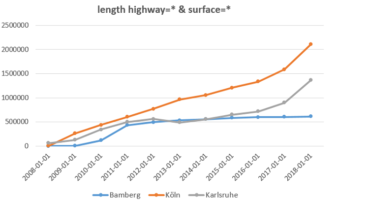
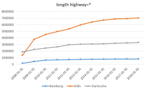
The first two diagrams show the length of OSM ways in meters tagged with the key highway (1) and those with the keys highway and surface (2).
(1)
(2)
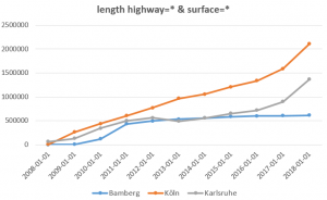
When we compare these two charts, we can see that the level of saturation of the curves (when there is no more significant incline) is reached at different points in time, or not at all. This effect occurs when not many edits of a certain tag are performed (but there is still overall mapping activity in that region, as explained in Neis et al. 2011, 2012, Barron et al. 2013), e.g. when most streets of a region most likely have already been mapped. Karlsruhe and Köln though have not reached their level of saturation yet when looking at the second diagram, in contrary to Bamberg, in spite of their active mapping community.
This situation is also reflected in the last diagram (3) showing the ratio between these graphs for every region.
(3)
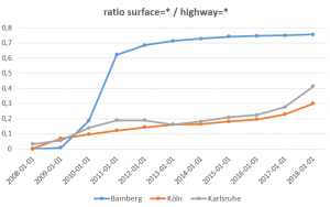
Here we clearly see that the ratio is highest for Bamberg. At the beginning of 2018, about 75% of the mapped streets in Bamberg had the surface tag. What is also visible here (like in diagram 2) is the positive trend of the other two graphs. More and more streets in Karlsruhe and Köln get the information about its surface added to them. This implies that the attributive completeness when looking at the tag surface=* is increasing for these cities. What we cannot say here though is if the added tags comply to defined standards. This topic was tackled in two other recently published posts, also dealing with the spatial version of compliance.
This blog post showed you how you can extract historical OSM data, visualize it and make simple statements about its quality and trend. You can also check out one of our dashboards, another easy to use component built on top of the ohsome framework. To contact us, just write us an email to info@heigit.org. Keep tuned for the next blog of the ohsome series, which is already in the pipeline and will take a look at varying mapping behaviors for different regions.